Unsupervised Image Classification
Note that the following is a simplified report with sections edited for simplicity. For a more in depth and comprehensive report, there is a PDF included within the repository.
Introduction and Background
Generating and labeling a large training set for training convolutional neural networks (CNNs) is costly and time-consuming. Moreover, internet-scale datasets are mainly unlabeled. To exploit the abundance of unlabeled images in the context of image classification, researchers have proposed extracting features from the images obtained via feeding the unlabeled images to a CNN [1][2][3][5][8].
There exist some unsupervised learning methods, like self-supervised learning and clustering-based methods. Self-supervision’s shortcoming is that it requires rich empirical domain knowledge to design pretext tasks. Among clustering-based methods, DeepCluster [3] is one of the most representative methods, which applies k-means clustering to the encoded features of all data points and generates pseudo-labels to drive an end-to-end training of the target neural networks. DeeperCluster[8] is an extension of DeepCluster[3], where it was trained on a larger dataset and a different neural network architecture. Researchers have also developed an approach that does not use traditional clustering methods like K-Means, instead opting to let the neural network do the clustering, making it a truly end-to-end deep learning approach[1]. In this report, we compare some of these unsupervised methods with the standard supervised methods for image classification.
Problem Definition
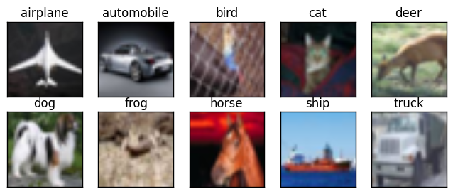
We try to solve how to label images of a dataset without their ground-truth labels. To train and evaluate our image classification algorithm, we will use the CIFAR-10 dataset [7] which contains about 60,000 examples covering 10 distinct classes. Using the labels provided by this dataset and the clusters determined by our algorithm, we will evaluate the accuracy of the learned clustering and compare the accuracy of the unsupervised methods against the supervised methods.
Data Collection / Pre-Processing
For the purpose of implementing this project, we will be using the Python programming language and the PyTorch deep learning library.
For these unsupervised image classification methods, it is absolutely crucial that you apply random and robust data augmentations. For the end-to-end[1], purely deep learning approach we implemented, you do one forward pass with one set of randomly applied data augmentations; then you use the CNN's predictions from this forward pass as the ground-truth. Then you do one more forward pass again with randomly applied data augmentations which, because they are random, are different from the first randomly applied data augmentations used to generate the psuedo-labels, and you train with the standard softmax cross-entropy loss. This process is done for each epoch of training. This forces the network to generalize to unseen data and not just memorize the dataset by using exactly its own past predictions on the exact same images used to make those past predictions.
We apply random changes in brightness, contrast, saturation, and hue, as well as random horizontal flipping and random center cropping with resizing with 50% chance. For the random color jitters, we used Pytorch's torchvision.transforms.ColorJitter (https://pytorch.org/docs/stable/torchvision/transforms.html) with the following parameters for brightness, contrast, saturation, and hue, respectively: (0.7, 1.3), (0.7, 1.3), (0.7, 1.3), (-0.2, 0.2).
For the unsupervised image classification, because DeepCluster[3] applies the sobel filter to the images before feeding to CNN, we also do this for the end-to-end approach[1]. We apply our data augmentations first; the sobel filter is applied last. We also try using the RGB images as input without the sobel filter, something DeepCluster did not do.
Below are some pictures that show our data augmentation and sobel filter being applied. We feed the gradient with respect to x and y concatenated channel-wise as input to the CNN, exactly the same as the deepcluster paper[3].
Gradient with respect to x after sobel filtering (vertical edges are brightest)
Gradient with respect to y after sobel filtering (horizontal edges are brightest)
One final transformation we do, is we upsample the 32x32 images to 64x64 using bilinear interpolation. We do this because the end-to-end approach[1] uses AlexNet. But 32x32 is too small for AlexNet, so we upsample by two.
For the traditional machine learning models such as SVM and Random Forests, we downloaded the dataset from the original website [2] and performed PCA dimensionality reduction while maintaining a variance of 99% the same way we did for the CNNs, then we flattened the images and fed them into the models to train. Note, we didn't apply the same augmentations applied to the dataset for the unsupervised method (random flips, color jittering, etc.) because the sklearn library does not provide "on-the-fly" data augmentation methods like pytorch does. We could have applied the augmentations to the training dataset, however, then we wouldn't have new augmentations with each forward pass, which we thought could be detrimental to the accuracy of the model. Thus we only applied the PCA dimensionality reduction method to the dataset, to improve training times and select the most important features from the images.
Modeling Methods
Unsupervised Modeling Methods
As mentioned in the previous section, the end-to-end approach[1] uses the predictions from the previous forward pass as the ground-truth labels for the current forward pass. According to the paper[1], this approach performs slightly better than DeepCluster[3] which is a deep learning approach as well, but instead of letting the CNN perform the clustering, it uses k-means clustering to generate pseudo-labels. For this report, we implemented the end-to-end unsupervised approach from the paper [1]. We did not implement the DeeperCluster approach and instead opted to just run their repo[8], changing the dataset from ImageNet to CIFAR10. Please note that the end-to-end approach[1] has not released their code yet, so we had to implement from scratch and from purely the authors' descriptions in their paper.
For the end-to-end approach, the pseudo labels in the current epoch are updated by the forward results from the previous epoch. Unlike DeepCluster/DeeperCluster where the embedding of each data point in the dataset should be saved before clustering, this end-to-end approach directly generates pseudo class IDs for each image on-the-fly during training. This makes it much faster to train. During the pseudo label generation, we directly feed each input image into the CNN classification model with softmax output and pick the class ID with highest softmax score as pseudo label. After the labels are generated, the model is trained on the new pseudo-labels like a supervised problem using the cross-entropy loss function. Different data augmentations are applied for each forward pass to force the model to generalize. While there is no explicit clustering in this approach like there is in Deep/DeeperCluster, it is actually clustering. The CNN is forced to learn how to properly cluster the images to minimize its loss. If the CNN at first gives the same label to a cat and an airplane, uses this as ground truth, and then different data augmentations are applied to these images, a change in the image could cause the CNN to now predict different labels for the cat and airplane, causing the loss to go up. Only if it properly clusters semantically similar images together, like cats with cats, will the model be robust to changes in the image, consistently predicting the same labels for semantically similar images, regardless of the data augmentations applied to those images. In traditional clustering, class centroids are dynamically found, the distance metric used is euclidean distance, and the optimal inter and intra cluster distances are used to properly form the clusters. In this classification approach, the centroids could be considered a set point of the true classifications for the images, and the distances between points are the cross-entropy loss. The “clusters” are formed naturally through whatever label the classifier predicts. However, there are some small implementation details to be aware of: In the initial training, it is common for the network to assign zero examples to a label, causing huge class imbalances. As mentioned in the paper[1], we resolve this by taking the label with the most examples, and giving half of these examples to the label with zero examples. Doing this, we found that this issue gets resolved during the first few epochs of training. We trained this method using AlexNet (same as original paper[1] and deepcluster[3]), VGG16 with batch normalization (same as deepcluster[3] and DeeperCluster[8]), as well as Resnet18, which was not used in any of the unsupervised image classification papers.
The DeepCluster architecture involves little domain knowledge. It simply adopts embedding clustering to generate pseudo labels by capturing the manifold and mining the relation of all data points in the dataset. In short, it iteratively groups the features with a standard clustering algorithm, their implementation uses k-means, and uses the subsequent assignments as supervision to update the weights of a convolutional neural network. The framework iteratively alternates between the k-means clustering and training the neural network. The neural network architectures for this approach are actually identical to normal supervised CNN models, such as AlexNet[10], ResNet[12], and VGG-16[9], which have already seen strong successes in supervised image classification. The authors also note that other clustering methods are also possible. An extension of the DeepCluster framework is the DeeperCluster[8] framework. It’s methodology is nearly identical to the DeepCluster framework, however its focus has been on processing larger datasets and distributive training. Because of this, it reduces the number of iterations to run while clustering, however sees very little change in performance compared to DeepCluster. The given default approach from the public code repository is the VGG-16 architecture.
Supervised Modeling Methods
For the traditional machine learning methods, we used the python library sklearn to implement the Random Forest, Support Vector Machine, K-Nearest-Neighbors, and Logistic Regression models. We applied PCA on the dataset for dimension reduction with a threshold of 99% variance; the original features of 3072 (which is 32x32x3 as each data point is an RGB image with a size of 32x32) are reduced to 658 features. We also did some hyperparameter tuning for these traditional machine learning methods. We used two different methods: Exhaustive grid search and Genetic Algorithm hyperparameter tuning.
For the Genetic Algorithm hyperparameter tuning, we used the DEAP evolutionary computation framework[11]. For a brief explanation of genetic algorithms, you start with a population of random potential solutions, then search and optimize the population through functions mimicking biological mating and mutation. Essentially, this method explores the problem space, without any prior knowledge of the problem, and optimizes for accuracy. This is oftentimes a great method for finding good parameters, but because the algorithm is seeded with random values, and has to explore the problems space, it takes a long time to converge. Also, if the initial population is too large, it will take a long time to evaluate, but if the initial population is too small there isn’t enough diversity in the solutions and we may get caught in local minima. While we were running this method, we determined it would likely take too long to converge for our purposes. For this reason, we instead switched to Exhaustive grid search for our hyperparameter tuning. This method takes in a hand-chosen list of potential hyperparameter values and finds the best combination of values that generate the best accuracy. This is the method we’ll use when we present in the results section. This method is preferable as we, as machine learning students, have a general idea of what good values are for hyperparameters, and thus we only need to find the best combination of these parameters, instead of the values of the parameters themselves, which is what this method provides. It should be noted that this method is still fairly slow, as exhaustively searching through all the combinations configured and training and evaluating all the models is still a time-consuming process.
For the supervised CNN approach, we used the standard softmax cross-entropy loss, using the same CNN architectures used for the unsupervised methods: AlexNet, VGG16 with batch normalization, and Resnet18. We did not end up applying hyperparameter tuning for the CNN-based approaches due to a lack of time and resources. Instead, we used the same hyperparameters as provided in the end-to-end paper[1] for both unsupervised and supervised approaches, instead focusing on running experiments between all these different methods and CNN architectures. We trained the CNN with SGD with momentum using the following hyperparameters: momentum 0.9, batch size 256, 1e-4 L2 weight decay, 0.5 drop-out ratio, and 1e-4 learning rate for 500 epochs, stepping the learning rate down to 1e-5 at 400 epoch. Similarly, when we compare our results to DeeperCluster, we used most of their initial parameters defined in their config file. However, due to hardware limitations, we did have to lower the batch size. However, DeeperCluster does its own data augmentation; therefore we only pass in the original unmodified CIFAR-10 dataset, not our augmented version.
Results
Traditional Machine Learning Supervised Methods
Among four models, SVM predicted well with the best accuracy of 48.5%. However, when we checked the accuracy of the prediction for the training set, we got 85.2% for it, which is a signal of overfitting. The Random Forest model also overfits with a huge difference of accuracy between testing and training set. On the other hand, Logistic Regression has less of a difference between testing set and training set accuracy, while maintaining a better than random chance prediction. From the table we see that the model usually finds four correct labels out of ten data points without overfitting, but the low accuracy on the training set is a sign of severe underfitting. One reason for why we are seeing overfitting and underfitting is that we have flattened the images in order to train them, so in reality we are training on the pixel values in the images. This is similar to how a dense neural network trains as well, however, because there are so many values with no particular information by themselves, the models likely overtrain on the images by deciding that certain pixels are the cause of their class, which causes it to perform poorly when generalizing. In contrast, the reason why CNNs have seen such wild successes in the recent years is because instead of just training on pixel values, it inherently does feature extraction and actually creates feature maps through its layers, which gives the network a better “understanding” of the images instead of just the pixels. It also reduces the chance of overfitting, as there are less parameters and the data points are combined together to form the feature maps.
For a better performance of each model, we tuned the hyper-parameters using sklearn's Exhaustive grid search method, GridSearchCV, which looks for a set of hyper-parameters giving the best accuracy as mentioned earlier. Naturally, there can be many different combinations of hyper-parameters for each model, causing this method to have a huge search space. Moreover, training each model with a set of hyper-parameters takes a long time in this method, depending on the performance of the machines we run them on. Therefore, we hand-picked a limited set of hyper-parameter candidates that are diverse enough to show how the models perform differently.
For Random Forest, we used the following lists of parameters to find the best precision and recall values.
Number of estimators: [10, 100, 200, 500, 1000, 5000]
Minimum number of datapoints per split: [0.1, 0.3, 0.5, 2]
Minimum number of datapoints per leaf: [0.1, 0.3, 0.5, 2]
Criterion: [entropy, gini]
As it has a larger number of estimators, the accuracy became better, but the time cost to train the model also became more expensive. For the best result, adjusting the minimum number of samples per leaf and the minimum number of samples per split played an important role as they may cause overfitting once the values become bigger than enough. The following set of parameters gave the best result with 0.355 as the accuracy, precision and recall:
Number of estimators: 5000
Minimum number of datapoints per split: 2
Minimum number of datapoints per leaf: 0.1
Criterion: gini
For k-Nearest Neighbors, we built models with all combinations of the following parameters.
Number of neighbors: [2, 4, 5, 7, 10]
Weights: [uniform, distance]
Algorithm: [auto, ball_tree, kd_tree, brute]
p (power parameter for the Minkowski metric.): [1,2,3]
The exhaustive grid search returned the optimal parameters (shown below) with an F1 score of 0.12:
Number of neighbors: 2
Weights: uniform
Algorithm: auto
p (power parameter for the Minkowski metric.): 3
For Logistics Regression, we built models with all combinations of the following parameters.
Penelization: [l2, none]
Tolerance for stopping criteria: [0.01, 0,001, 0.0001, 0.00001]
Inverse of regularization strength: [0.5, 1, 10, 100, 1000]
Optimization algorithm: [lbfgs]
Maximum iterations for optimization: [10, 25, 50, 100, 150, 200, 500, 1000, 10000]
We chose the optimization algorithm to be Limited-memory BFG (lbfgs) since it handles polynomial loss for multiclass datasets, and it works well with many variables as CIFAR10 dataset has a lot of features that are the flattened pixels of images. Since the chosen optimization algorithm only takes the l2 norm to penalize for regularization, we wanted to compare how the result would be different with/without the regularization. The rest parameters such as the number of iterations, the size of regularization are decided to have general various values. As a result of it, all the sets of the parameters gave the same rate of 0.40 for accuracy, precision and recall.
For SVM, the combination of parameters are as follows:
Kernel : [linea, sigmoid, rbf]
gamma : [0.001, 0.0001]
C : [100, 1000]
We tuned the hyper-parameters separately for precision and recall. Overall, the rbf kernel had the highest accuracy score for precision and recall, therefore the highest f1-score of 0.52 with the set of parameters below:
Kernel : rbf
gamma : 0.001
C : 100
We can argue why these values for gamma and C help the model perform better on our dataset. As mentioned in the documentation of RBF kernel for SVM, gamma defines how far the influence of a single training example reaches, and C behaves as a regularization term in the SVM. Smooth and simple models have lower gamma values, and can be made more complex by increasing the importance of classifying each point correctly, which means higher C values.
CNN Supervised Methods
Below are our results training AlexNet, Resnet18, and VGG16 with batch normalization using the supervised softmax cross-entropy loss. Please note that we re-trained AlexNet with more aggressive data augmentation since our midterm report, hence why the results for AlexNet are different (the model improved!).
The data fed to the CNN were RGB images going through all the randomly applied data augmentation approaches mentioned earlier except for the sobel filter which will only be used for training the unsupervised approaches. The model was trained with the same hyperparameters as the end2end unsupervised approach we are trying to implement[1].
Compared to the traditional machine learning approaches, it didn’t overfit too badly, and it did better than all of them for the test set but actually did worse on the training set compared to Random Forest and SVM. This suggests that the CNN's may actually be underfitting, and there is still much room for improvement.
AlexNet performed the worst as expected because it is the simplest architecture without any normalization layers. Surprisingly, VGG16 with batch normalization outperformed Resnet18. The point of residual blocks was to help with the vanishing gradient problem to allow for deeper and deeper networks to learn more and more complicated functions. Most likely, CIFAR10 is a simpler and smaller dataset that does not require a more complicated architecture to properly learn.
You may see a graph of our tensorboard output for AlexNet training here as well as a visualization of some of our network’s predictions:
Figure 1: Tensorboard Cross-Entropy Loss vs Number of Training Iterations (blue is validation loss; orange is training loss).
Figure 2: Visualization of final predictions on training and validation set at end of training using tensorboard
Unsupervised CNN Methods
End-to-End Deep Learning Approach
Initial Training; Psuedo-Labels before and after Re-balancing
Figure 3: This image shows what the psuedo-labels look like initially during training before and after re-balancing.
Figure 4: However, as training moves toward completion, the model learns a relatively balanced dataset, as it should, because CIFAR10 training set is almost perfectly balanced among the 10 classes.
Figure 5: These are the training (orange) and validation (blue) loss curves when training end-to-end approach using AlexNet with RGB images. Ignore the validation curve. With this unsupervised method, as the ground-truth labels are the predicted labels from the previous forward pass, there is no such thing as a validation set. The validation curve in this case is showing how the model performs on the original test set, which is meaningless in this case because the psuedo-labels are not going to match the original labels. However, you can see that the training loss converges rather nicely; it actually converges to a similar level as the supervised training.
Figure 6: Some predictions visualized by tensorboard for the unsupervised training. You can see that the predictions match the ground-truth. However, the two examples on the left are both frogs, but the model labeled the ground-truth for one of them as airplane and the other as cat, showing how the model is not learning the best clustering.
For the unsupervised methods, it actually doesn't make sense to directly compute top1-accuracy because the model learns its own semantically unique labels, and it is not possible to extract the original ground-truth labels from these learned labels. By definition, in unsupervised learning, there is no such thing as ground-truth labels. The only way we could directly compare the unsupervised approaches with the supervised approaches directly is if the unsupervised approach did such a good job at clustering, that it predicts one unique label for each class. Specifically, if we feed all the examples of airplanes from the training set to the model, we would look at the label it chose most often, say label 2, and assign label 2 to airplane. Then when we feed all the examples of birds from the training set to the model, and the most chosen label should NOT be 2. It should not be a label that was already chosen. However, this is actually what happened with our end-to-end implementation. The model predicted label 2 as the most likely label for both birds and airplanes, meaning when the model predicts 2, it could be a bird or an airplane; there is no way for us to know which one it is. Even if you know airplane is more likely than bird when it predicts label 2, and you choose to associate the 2nd most likely label with bird which may be label 4, another class name could be more likely to be associated with label 4. So you keep going down to the 3rd most likely, to the 4th most likely, until you reach a label that hasn't been chosen by another class, but this label was only chosen, say, 5% of the time when shown all the training images of birds, compared to choosing the label 2 40% of the time. Obviously, the model thinks label 2 belongs to bird as it chose it 40% of the time, but label 2 was even more likely to be chosen when shown airplanes. So the model also thinks label 2 belongs to airplane. In our opinion, this problem is inherently ambiguous and is impossible to resolve in a way that makes sense. We even confirmed by emailing the authors of the end-to-end paper[1] that there is no objective way to resolve this ambiguity. This is why in these unsupervised image classification papers, they use normalized mutual information (NMI) to quantify how good of a clustering their approach did. And they do linear probing of their CNN to train a linear classifier using their trained CNN as a feature extractor. For example, they would freeze the convolutional layers and then attach some fully-connected layers to convolutional layer 3, to convolutional layer 4, etc and only train those full-connected layers for a supervised task. This allows us to quantify how good of a representation the model learned from the unsupervised task, how useful those learned features are. And then with these trained models, we can evaluate top1-accuracy. We follow these same evaluation metrics: We evaluate how good of a clustering the CNN learned by using NMI, and we do linear probing for our trained AlexNet, Resnet18, and VGG16_bn end-to-end unsupervised models, training it on the CIFAR10 dataset. We also use these evaluation metrics to compare whether it is better to train with sobel-filtered images or the original RGB images.
Normalized Mutual Information
We used sklearn's implementation of normalized mutual information (https://scikit-learn.org/stable/modules/generated/sklearn.metrics.normalized_mutual_info_score.html) which is the same function used in the deepcluster repo[3]. The metric tells us how much mutual information is shared between the ground-truth clusters and the predicted clusters, which in our case, are our ground-truth labels and the predicted labels from our model. The metric ranges from 0-1, with 0 meaning no mutual information between the groups of clusters (worst) and 1 meaning perfect correlation between the groups of clusters (best).
According to Table 1 from the original end-to-end paper[1], they were getting an NMI of around 0.38-0.42 when using AlexNet trained on the ImageNet dataset which consists of millions of images and 1000 classes. Our AlexNet results are much worse probably because we trained on the much smaller CIFAR10 dataset which only has 60,000 images and 10 classes. Most likely, if we had a larger variety of data, the network would have had an easier time learning distinct clusters.
Resnet18 did slightly better than AlexNet. But most surprisingly, VGG16_bn did the best by far, scoring even higher than the 0.38-0.42 in the paper[1]. Once again, like with the supervised CNN approaches, VGG16_bn outperformed Resnet18.
Linear Probing
For AlexNet, we probed from the third and fifth (last) convolutional layers. For Resnet18, we probed from the third and fifth (last) residual blocks. For VGG16_bn, we only probed from the very last convolutional layer. We would have liked to run more experiments, but we did not have the time and resources to do so. When training these linear probes, we used the same data augmentations that was used to train all other CNN experiments. The results of our linear probing experiments as shown below:
Please note that we were using these CNN architectures as out-of-box as provided by PyTorch. We accidentally forget to disable the non-linear activation functions in the classifier portion of these CNN's for AlexNet and VGG16_bn. So they were technically not "linear" probing. And we did not have time to re-train so many experiments. Thankfully, Resnet18 only uses one fully-connected layer as its classifier and is therefore fair to compare with the original end-to-end paper[1].
If you look at Table 1 and Table 2 of the original end-to-end paper[1], they used their feature extractors trained unsupervised on Imagenet to linearly probe on the PASCAL VOC dataset. They got around 0.38-0.41 top1-accuracy on the test set. We also got about 0.40 top1-accuracy for our Resnet18 when linearly probling from block 5 for both RGB and Sobel images. We got much lower accuracy when probling from block 3; the model underfit so poorly, the training set accuracy was actually slightly worse than the test set accuracy. We believe this is most likely due to the nature of residual blocks and skip connections; it probably doesn't make sense to only use part of a resnet backbone. It's possible the earlier blocks' weights were learning something closer to an identity function and were therefore not useful. We do not see such a stark difference in accuracy when comparing different probes in our AlexNet experiments or in the original end-to-end paper's experiments[1].
Another interesting thing to note is that for AlexNet, probing from a deeper layer actually gave worse results, the same as the paper[1]. We believe this is likely due to the fact that the shallower layers have more features to use for classification than the deeper layers. But the trade-off is that the features are not as rich. If you look at the results from Table 1 of the deepcluster paper[3], their linear probe's top1-accuracy peaks in the middle layers as well.
It seems that using RGB images gives just as good but usually better results than using images after sobel filtering to train the model. This makes sense as the RGB images give more information and therefore more useful features than the gray-scale sobel-filtered images which only have edge information.
While the unsupervised methods did underperform their supervised CNN counterparts, our best unsupervised method, Resnet18 probed from block 5, was on par or outperformed all the traditional machine learning methods except for SVM.
Finally, it's worth noting that while VGG16_bn performed better as measured by NMI, it actually performed worse with the linear probing when compared fairly to Resnet18 probed from block 5, even though VGG16_bn was accidentally trained with a non-linear classifier while Resnet18 only had one linear full-connected layer as its classifier. Also, while AlexNet performed the worst as measured by NMI; it performed the best in the linear probing. We are not sure why this happened.
DeeperCluster
We compared the results to DeeperCluster. Unfortunately, there were issues found while training, we could only complete 3 epochs while the expected number of completed epochs was 100. There appear to be known issues with DeeperCluster’s current implementation that we have also run into while trying to run their code. (https://github.com/facebookresearch/DeeperCluster/issues/18). Because of this, our accuracies are extremely poor, and we believe our models have not enough time to train and converge. As you can see, after the 3rd epoch of training we reach about 9% training accuracy, which is what we would expect from random chance from the CIFAR-10 dataset. It should be noted that since these methods don't train using labels, having an accuracy on the test set doesn't make much sense. The "labels" the models are trained on are produced by the models themselves. Because the labels are dynamically defined, the models' predicted label may not be the same as the true label's definition, but it ultimately classified the image correctly. So the traditional method of comparing the labels of the prediction to the true labels in the test set cannot apply in this scenario. The proper way to evaluate these models would be to look at what they consider each psuedo-label, then determine which true label closest matches the pseudo-label, then determine if the prediction is correct. This would likely be a time consuming manual process. Because of this, it should be noted that our evaluation metrics are a little different from the end-to-end method. We use k-means and explicitly cluster, so we can forcefully create the correct number of classes. So the empty class problem in the end-to-end approach is somewhat mitigated. However, there are no guarantees that the labels assigned to each image in the cluster match the true ground truth labels from the original dataset. Nothing should be inferred from these results, as we could not train to completion, however this is meant more to highlight our attempts to compare our results to other state of the art literature and act as an example of a model that did not converge.
Discussion
Our traditional supervised learning models always severely overfit or underfit, even though we tuned the hyperparameters. Specifically, our SVM and Random Forest models were overfit and our kNN and Logistic Regression models were underfit. Some ways we could improve our overfit models are by getting more training data, using fewer features, or using an early stopping mechanism to prevent the model from getting too complex. An example of this could be reducing the number of trees in our Random Forest or by pruning certain trees. In order to improve our underfit models we could try to use more features, so not using PCA dimensionality reduction could help these models. However, the likely case is that these classifiers/algorithms simply aren't very good for this type of problem.
Our supervised CNN approach performed predictably better across the board for all CNN architectures against all traditional machine learning approaches.
Our unsupervised CNN approaches performed comparably to the traditional machine learning approaches. We expected them to perform worse than the supervised neural network, but better than the traditional machine learning models. The only exception was the DeeperCluster experiment, which due to hardware limitations, we could not train to completion. Some other potential reasons for why our DeeperCluster result performed poorly is that the datasets DeeperCluster was originally trained on were much larger and diverse. For example, nearly all state of the art convolutional neural networks are trained on the ImageNet dataset[13], which is composed of over 14,000,000 images with varying sizes. Deep/DeeperCluster were trained on the YFCC100m dataset [14], which was over 100,000,000 images of varying sizes. In comparison, the CIFAR-10 dataset is only comprised of 60,000 images, all of which are extremely tiny, only 32x32 pixels. In order for some of our neural network architectures to work on the CIFAR-10 dataset, we had to upsample our image through interpolation, but it may be a sign that these architectures weren’t meant for tiny images in the first place. Similarly, when we perform data augmentations such as random crops and the sobel filter, since our images are already so tiny and somewhat distorted, our augmentations might actually be having a negative impact on the model’s training. It may cause the models to believe that some important features are actually noise. However, we do want to highlight that data augmentations in general are the recommended way to improve accuracies for CNNs. Even in our project, after applying data augmentations, our accuracies for the supervised AlexNet architecture improved.
Potential ways that could increase the accuracy for all the CNN models are finding ways to further expand the dataset or changing which features to use. If we wanted to expand the dataset in an advanced state of the art way, GANs have seen great success with producing similar, yet different images, so if a GAN was used to produce similar looking images to those in the CIFAR-10 dataset we could expand the training data. However, GANs are again a very computationally expensive approach. The more traditional way would be to perform more data augmentations such as different rotates and feature extractions. Another potential reason is that our models haven't finished converging. For DeeperCluster specifically, we couldn't finish the training all the way through so we know it didn't converge properly, which explains some of the poor results. Similarly, our end-to-end implementation's loss is a bit tricky as the "truth" labels often change due to the psuedo-label generation process. It becomes difficult to tell when our model has properly converged.
Looking into the current state of the art performance on the CIFAR-10 dataset, we find that the authors [15] that currently hold the highest accuracy of 99.7% did not actually make many model modifications, but rather used a normal ResNet[12] implementation. Their paper rather focused on highlighting the importance of data augmentations, and showing that optimizing the loss function alone while training is not enough.
Another simpler way to possibly improve the unsupervised approaches is for each image, we can generate some K number of augmented images. Then whatever psuedo-label the model assigns to the original image, we also assign that same psuedo-label to the K number of augmented images. This may help the model learn the differences between the different classes, especially if the augmentations include random perspective transformations which cause the image to be viewed from different angles. It would not make sense to let the model choose the psuedo-label for these K augmented images, as we know these images must be of the same label as the original image. By doing this, we are, in a way, providing a supervisory signal.
Conclusion
We were able to solve the initial problem of classifying images without their labels by implementing the end-to-end paper[1]. We were able to recreate a model that doesn't require domain knowledge, and run a state of the art model that also solves the problem. While we weren't able to successfully replicate all of their results, we have determined that such a method is very possible and useful. However, when compared to existing supervised methods with labels, our model accuracies fall short as expected. We have also shown how traditional machine learning models are capable of solving the CIFAR-10 dataset, but are likely to be overfit. Whereas in comparison, supervised convolutional neural networks are able to reach high accuracies without overfitting.
References
[1] Weijie Chen, Shiliang Pu, Di Xie, Shicai Yang, Yilu Guo, & Luojun Lin. (2020). Unsupervised Image Classification for Deep Representation Learning.
[2] Krizhevsky, A. (2012). Learning Multiple Layers of Features from Tiny Images. University of Toronto. Link to Dataset: https://www.cs.toronto.edu/~kriz/cifar.html
[3] Mathilde Caron and Piotr Bojanowski and Armand Joulin and Matthijs Douze (2018). Deep Clustering for Unsupervised Learning of Visual Features. CoRR, abs/1807.05520. Code Repository Link: https://github.com/facebookresearch/deepcluster
[4] Gabriella Csurka, Christopher R. Dance, Lixin Fan, Jutta Willamowski, & Cédric Bray (2004). Visual categorization with bags of keypoints. In Workshop on Statistical Learning in Computer Vision, ECCV (pp. 1–22).
[5] Jeff Donahue and Philipp Krähenbühl and Trevor Darrell (2016). Adversarial Feature Learning. CoRR, abs/1605.09782.
[6] Piotr Bojanowski, & Armand Joulin. (2017). Unsupervised Learning by Predicting Noise.
[7] CIFAR-10 and CIFAR-100 datasets. (2009). Toronto.Edu
[8] Mathilde Caron, Piotr Bojanowski, Julien Mairal, & Armand Joulin. (2019). Unsupervised Pre-Training of Image Features on Non-Curated Data. Code Repository Link: https://github.com/facebookresearch/DeeperCluster
[9] Karen Simonyan, & Andrew Zisserman. (2015). Very Deep Convolutional Networks for Large-Scale Image Recognition.
[10] Krizhevsky, A., Sutskever, I., & Hinton, G. (2012). ImageNet Classification with Deep Convolutional Neural Networks. In Advances in Neural Information Processing Systems (pp. 1097–1105). Curran Associates, Inc.
[11] Félix-Antoine Fortin, Fran\ccois-Michel De Rainville, Marc-André Gardner, Marc Parizeau, & Christian Gagné ( 2012 ). DEAP: Evolutionary Algorithms Made Easy Journal of Machine Learning Research , 13 , 2171–2175 .
[12] Kaiming He, Xiangyu Zhang, Shaoqing Ren, & Jian Sun. (2015). Deep Residual Learning for Image Recognition.
[13] Deng, J., Dong, W., Socher, R., Li, L.J., Li, K., & Fei-Fei, L. (2009). ImageNet: A Large-Scale Hierarchical Image Database. In CVPR09.
[14] Bart Thomee and David A. Shamma and Gerald Friedland and Benjamin Elizalde and Karl Ni and Douglas Poland and Damian Borth and Li-Jia Li (2015). The New Data and New Challenges in Multimedia ResearchCoRR, abs/1503.01817.
[15] Pierre Foret, Ariel Kleiner, Hossein Mobahi, & Behnam Neyshabur. (2020). Sharpness-Aware Minimization for Efficiently Improving Generalization.
Unsupervised Image Classification